Introduction to Bootstrapping in Data Science — part 2

In the first part of the series, we described how to estimate the confidence interval of almost any feature in a broader population, using just a random sample and a simple iterative algorithm known as bootstrapping. This method has decisive advantages over traditional statistical methods: it is a sort of one-fits-all approach that allows us to face challenging problems with a few lines of code. Interestingly, it also breaks us free from theoretical frameworks, usually constrained by assumptions that may not hold in every possible situation. And, truth be told, there are many scenarios where we cannot rely on those well-known textbook solutions.

The good news is that bootstrapping may be easily applied to other settings such as two-sample problems and hypothesis testing. We will cover the former in this article and leave the latter for the third and last instalment of the series (so stay tuned!). In the first sections of this post, we will estimate the difference in means of two normal distributions where the variances are unknown and not equal using both parametric and bootstrapping approaches, as proof that both methods agree. Then, we will propose a more challenging problem for which there is not a simple parametric solution while bootstrapping can solve it without hassle.

Example 1.1: Traditional difference in means with variances unknown and not equal

Let’s imagine we have two populations that follow a normal distribution (a big assumption to begin with) with unknown means and variances. We also know that the variances are different from one another. In this scenario, we need to estimate the difference in the means and provide a reasonable confidence interval. Despite this is a somewhat unfavourable case of sample comparison, it is also a well-known problem that you may look up in your favourite statistics textbook (Figure 1):

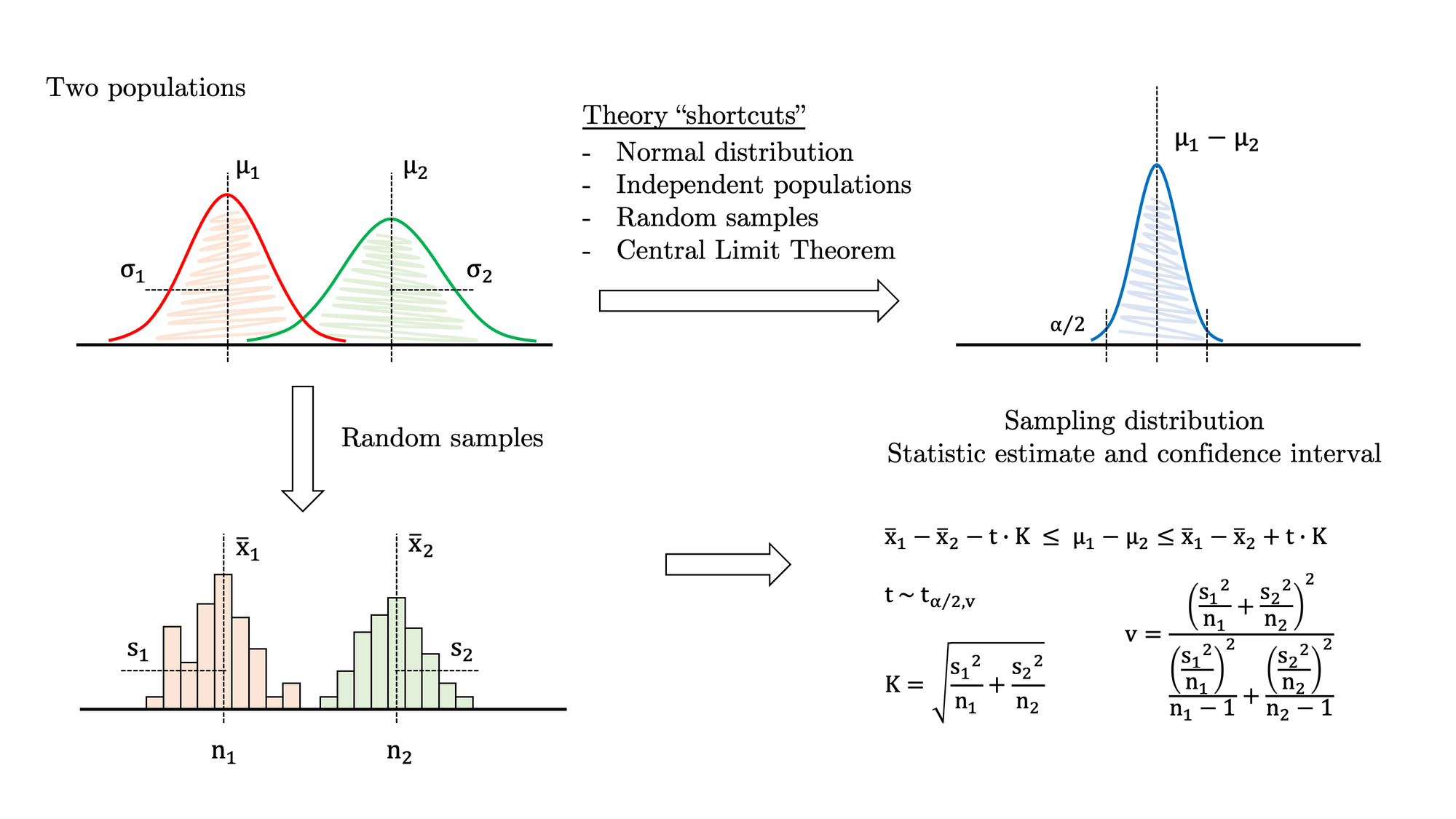
Some of the equations above are relatively dense, but nothing we cannot handle in Python. Besides, if the sample size is big enough, you may simplify the problem and switch to a z-statistic instead of a t-statistic (and get rid of the complex calculation of the degrees of freedom). In any case, let’s stick to the full-fledged formula and follow this procedure:

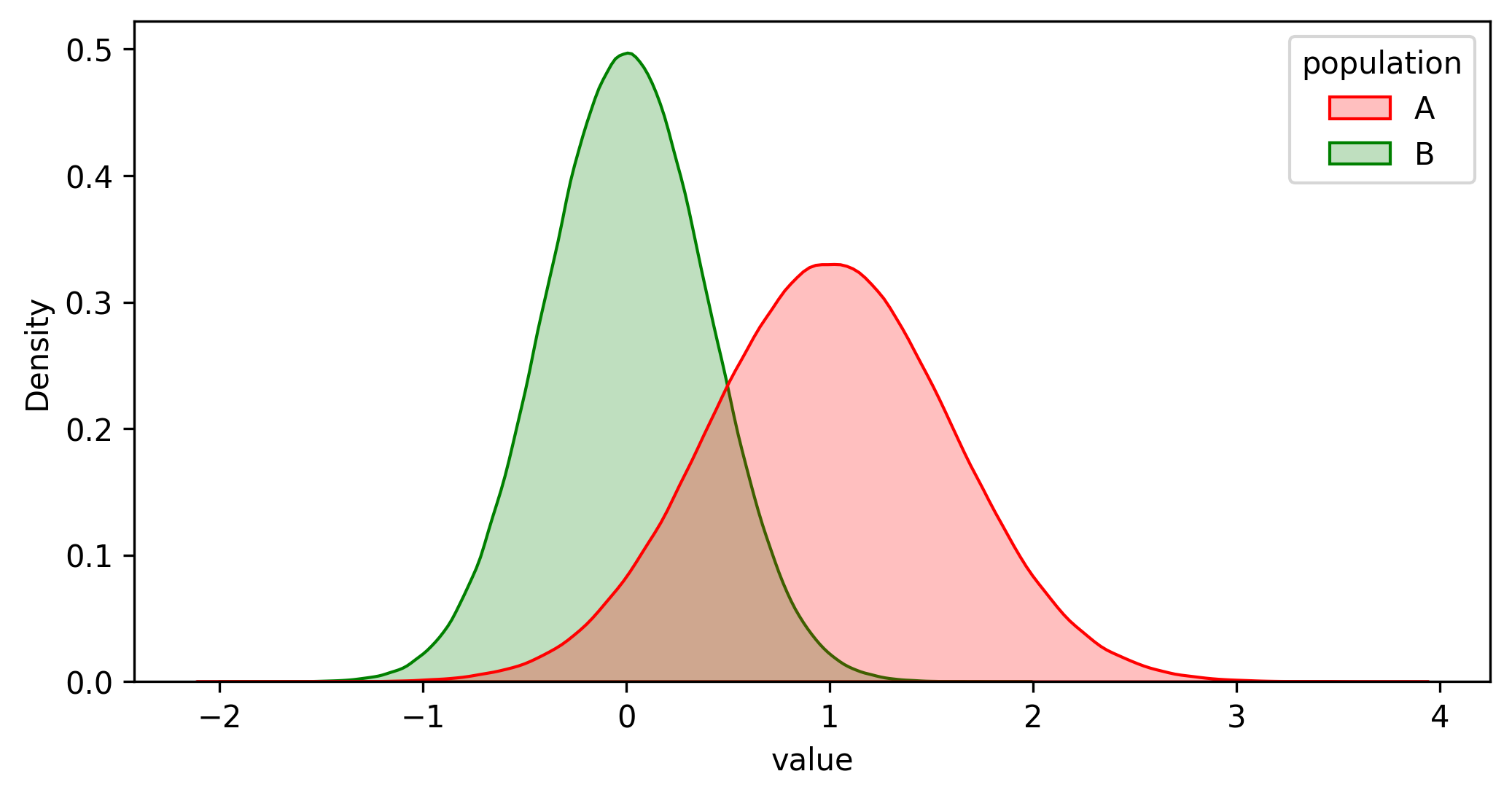
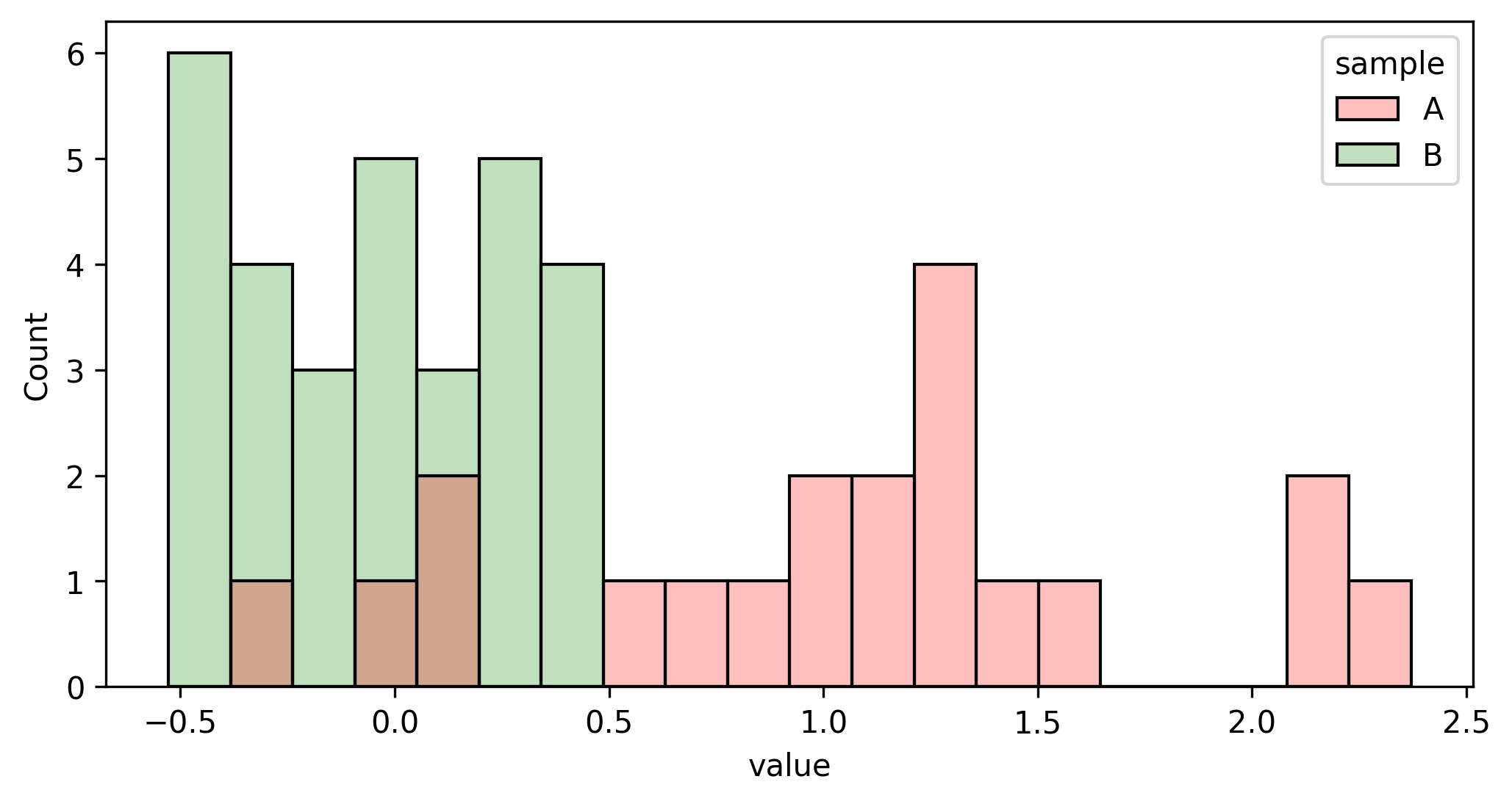
1. Draw a random sample from each population (see Figures 2 and 3).
2. Calculate the statistic and the confidence interval using the theoretical approximation shown in Figure 1.

This is a Python function that estimates the confidence interval:

from numpy import mean, sqrt, std
from scipy.stats import t

def difference_means_confidence_interval(sample1, sample2, alpha):
    """ calculate the confidence interval for difference in means unknown variance """
    
    # sample data
    n1, m1, s1 = len(sample1), mean(sample1), std(sample1)
    n2, m2, s2 = len(sample2), mean(sample2), std(sample2)

    # statistical stuff
    K = sqrt(s1**2/n1 + s2**2/n2)
    v = (s1**2/n1 + s2**2/n2)**2 / ((s1**2/n1)**2/(n1-1) + (s2**2/n2)**2/(n2-1))
    d = K * t.ppf(1.-alpha/2, v)
    
    # confidence interval
    diff = m1 - m2
    low  = diff - d
    high = diff + d
    
    # print results and return
    print(f'Difference={diff:.3f}')
    print(f'Confidence interval ({1-alpha:.0%}): [{low:.3f}, {high:.3f}]')
    return low, diff, high

difference_means_confidence_interval(sample1, sample2, alpha=0.05)

Difference=1.092
Confidence interval (95%): [0.741, 1.444]

With 95% confidence, we can assure that the difference in means is greater than 0.741 and less than 1.444. This result is good enough as the actual value is 1.

Example 1.2: Same problem solved with bootstrapping

And here comes the bootstrapping function. The algorithm is very similar to the one-sample version described in detail in the first article of the series:

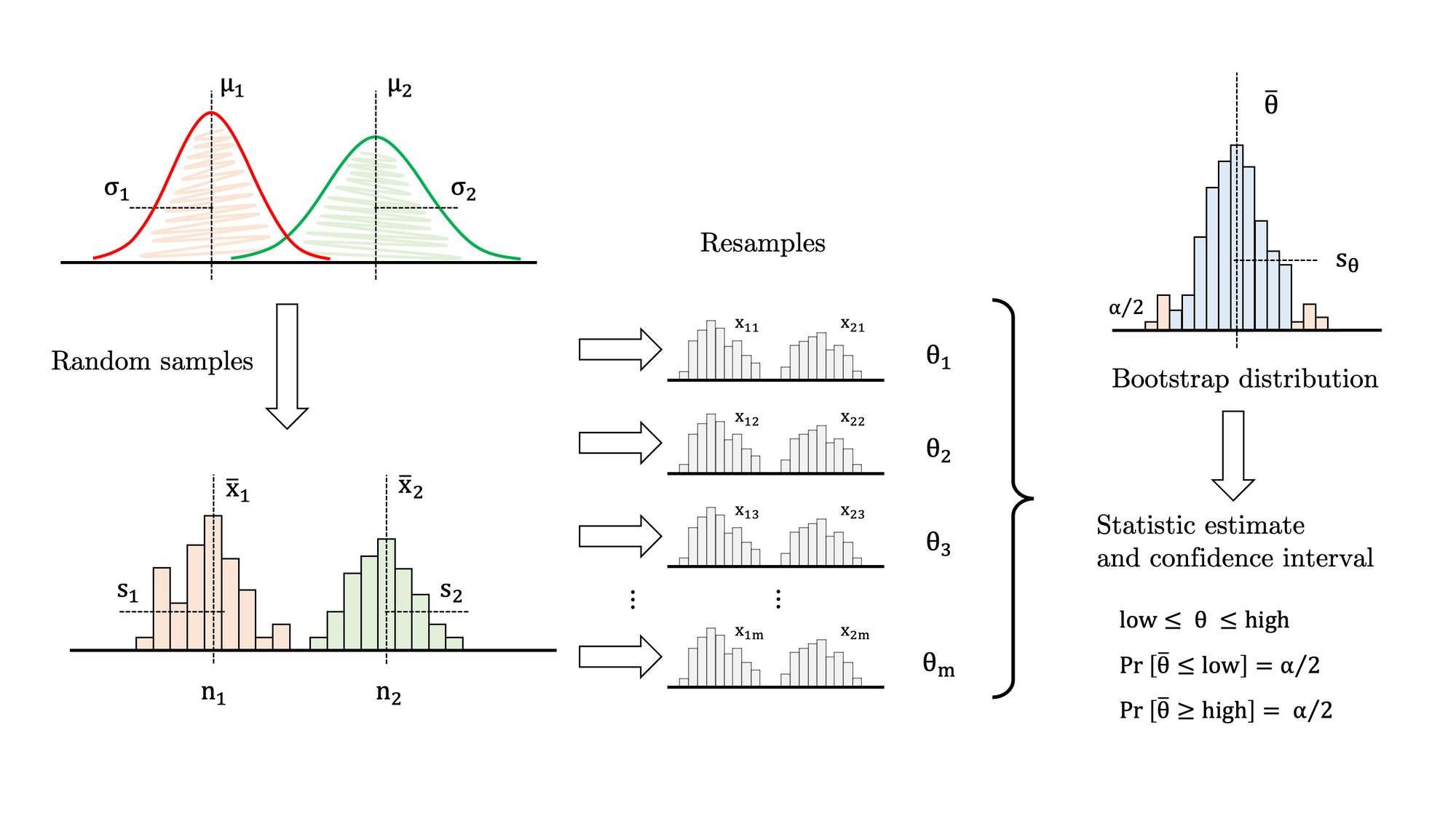
1. Draw samples A and B from both populations (see Figures 2 and 3).
2. Draw a resample with replacement from the original sample A, with exactly the same size.
3. Draw a resample with replacement from the original sample B, with exactly the same size.
4. Calculate the estatistic over both resamples (in this case, difference in means).
5. Store the statistic in a list.
6. Go to 2. Repeat thousands of times.

import seaborn as sns

def bootstrap2_fn(sample1, sample2, fn, iterations, alpha):
    """ bootstrap any given function over two samples """
    
    # original samples and statistic
    n1 = len(sample1)
    n2 = len(sample2)
    sample_fn = fn(sample1, sample2)
    
    # bootstrap algorithm
    bootstrap_dist = []
    for i in range(iterations):
        resample1 = np.random.choice(sample1, n1, replace=True)
        resample2 = np.random.choice(sample2, n2, replace=True)
        estimator = fn(resample1, resample2)
        bootstrap_dist.append(estimator)
    
    # calculate mean, standard error and bias
    bootstrap_mean  = np.mean(bootstrap_dist)
    bootstrap_se    = np.std(bootstrap_dist)
    bias = sample_fn - bootstrap_mean
    
    # calculate bootstrap percentile confidence interval
    high   = np.quantile(bootstrap_dist, 1-alpha/2)
    median = np.quantile(bootstrap_dist, .5)
    low    = np.quantile(bootstrap_dist, alpha/2)
        
    # plot bootstrap distribution
    sns.histplot(bootstrap_dist, stat='density')
    sns.kdeplot(bootstrap_dist)
    
    # print results and return
    print(f'{n1=} {n2=} {iterations=}')
    print(f'{sample_fn=:.3f} {bootstrap_mean=:.3f} {bias=:.3f} {bootstrap_se=:.3f}')
    print(f'Confidence interval ({1-alpha:.0%}): [{low:.3f} ... {median:.3f} ... {high:.3f}]')
    return low, median, high


# difference in means
diff_means_fn = lambda x1, x2: mean(x1) - mean(x2)
   
# bootstrapping
bootstrap2_fn(sample1, sample2, diff_means_fn, iterations=10000, alpha=0.05)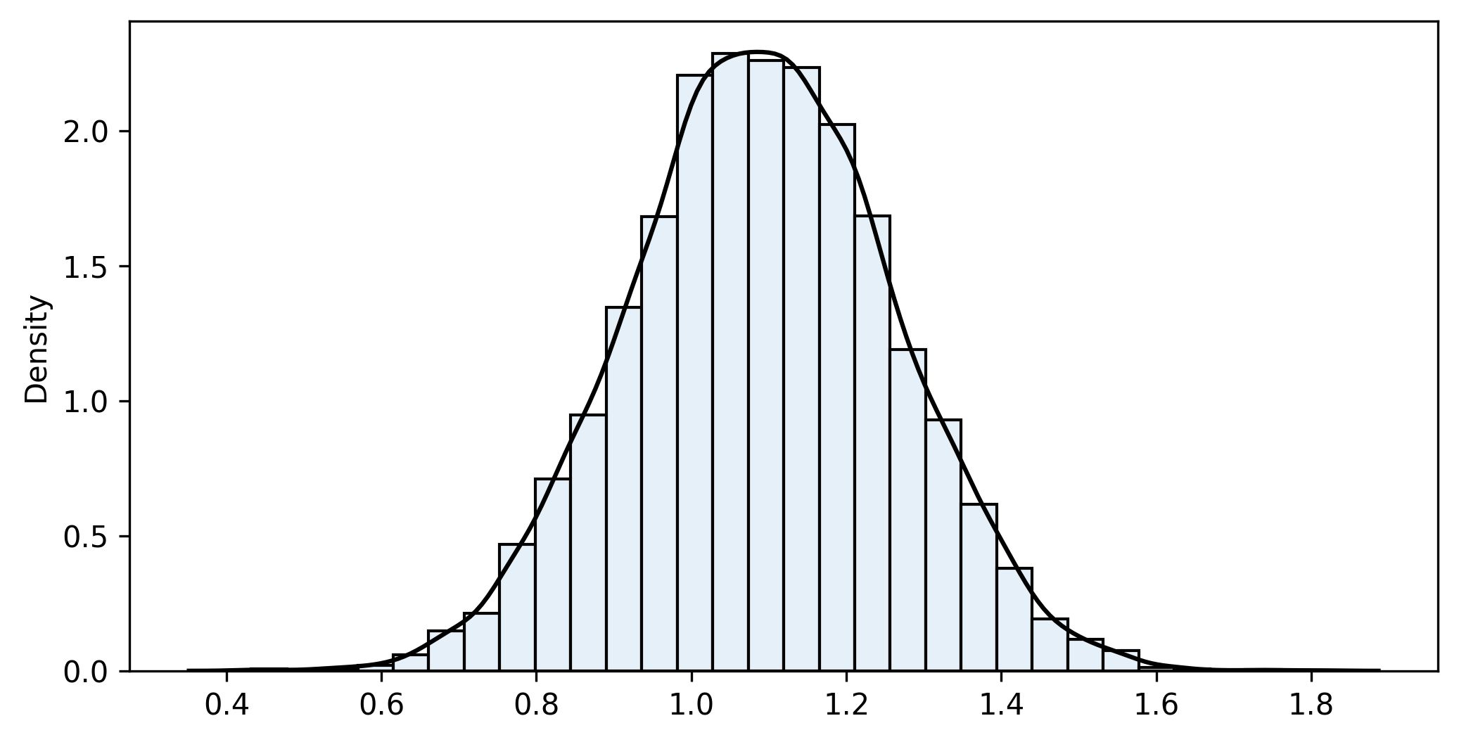

n1=20 n2=30 iterations=10000
sample_fn=1.092 bootstrap_mean=1.091 bias=0.002 bootstrap_se=0.169
Confidence interval (95%): [0.762 ... 1.090 ... 1.418]

The distribution of the values in the list is the bootstrap distribution, which approximates the theoretical sampling distribution. Generally, it is centred on the value of the statistic in the samples (not the populations), allowing for a small bias. It is always a good idea to plot it and check whether it is approximately normal. Next, we compute the non-parametric bootstrap percentile confidence interval. That is, pick the two quantiles that enclose under the bootstrap distribution the area required for your confidence level.

Both results, parametric and bootstrap, are close enough. However, note that the parametric approach is specifically tailored for this problem, while bootstrapping is entirely generic. What happens if we need to estimate, for example, the difference in variances or any other custom measure? For the parametric method, we have to look for a different set of equations (should they exist). Conversely, bootstrapping only requires a minor update in the code. The following section will describe precisely these changes with another example.

Example 2: salary comparison between two firms

Let’s imagine that we would like to compare the salary distribution of two competing companies. Working for either of them is really tempting and, as a job prospect, there is not any notable difference apart from compensation. Unfortunately, they do not disclose this sort of information, but we managed to get our hands on two random samples:

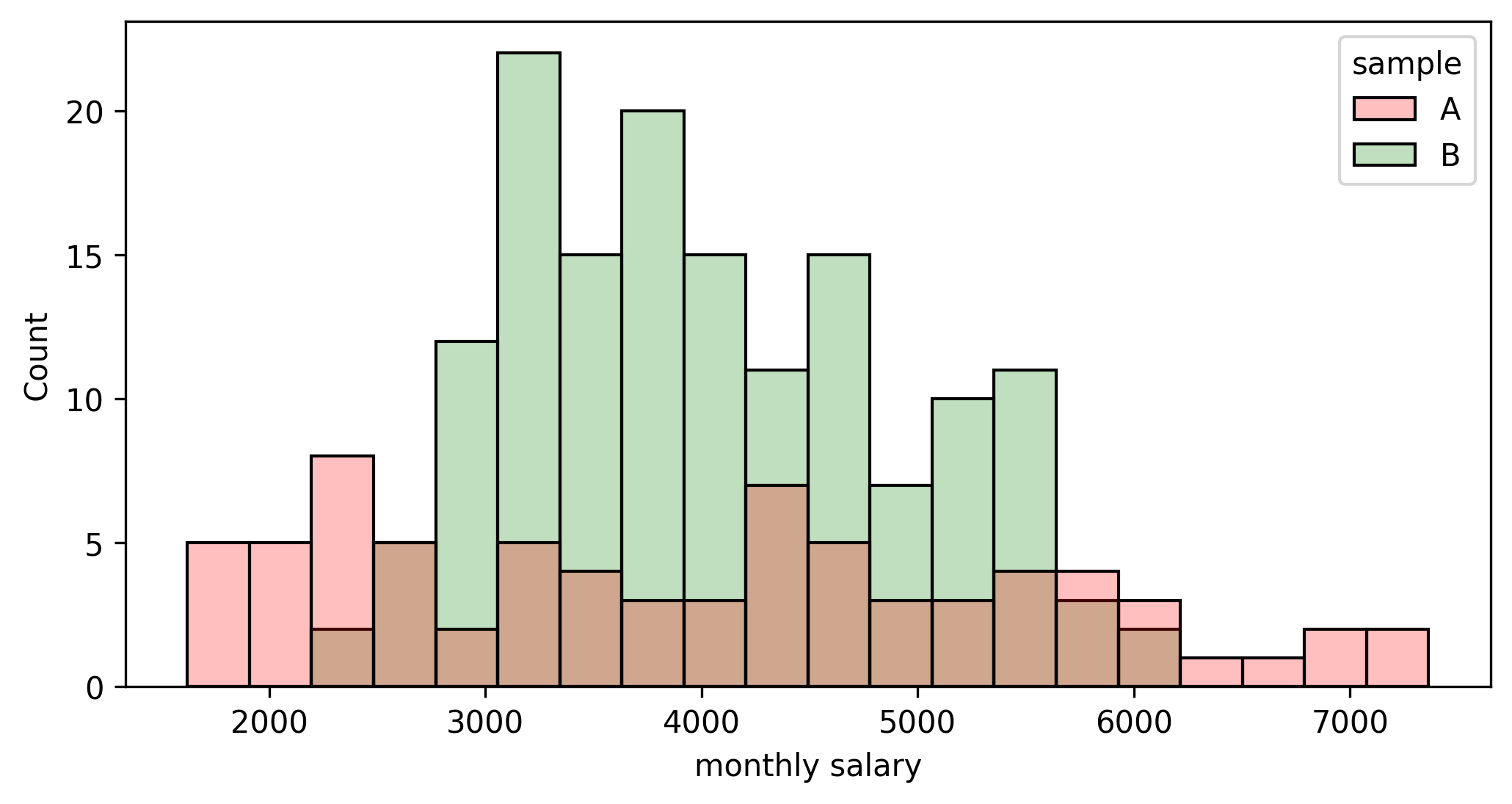
The first question is: “How do both means compare to each other?” Both traditional and bootstrapping approaches may solve this step, and the result is:

# estimate the difference in means
difference_means_confidence_interval(sample1, sample2, alpha=0.05)

Difference=-77.982
Confidence interval (95%): [-460.342, 304.377]

And with bootstrapping:

# difference in means
diff_means_fn = lambda x1, x2: mean(x1) - mean(x2)

# bootstrap function over two samples
bootstrap2_fn(sample1, sample2, diff_means_fn, iterations=10000, alpha=0.05)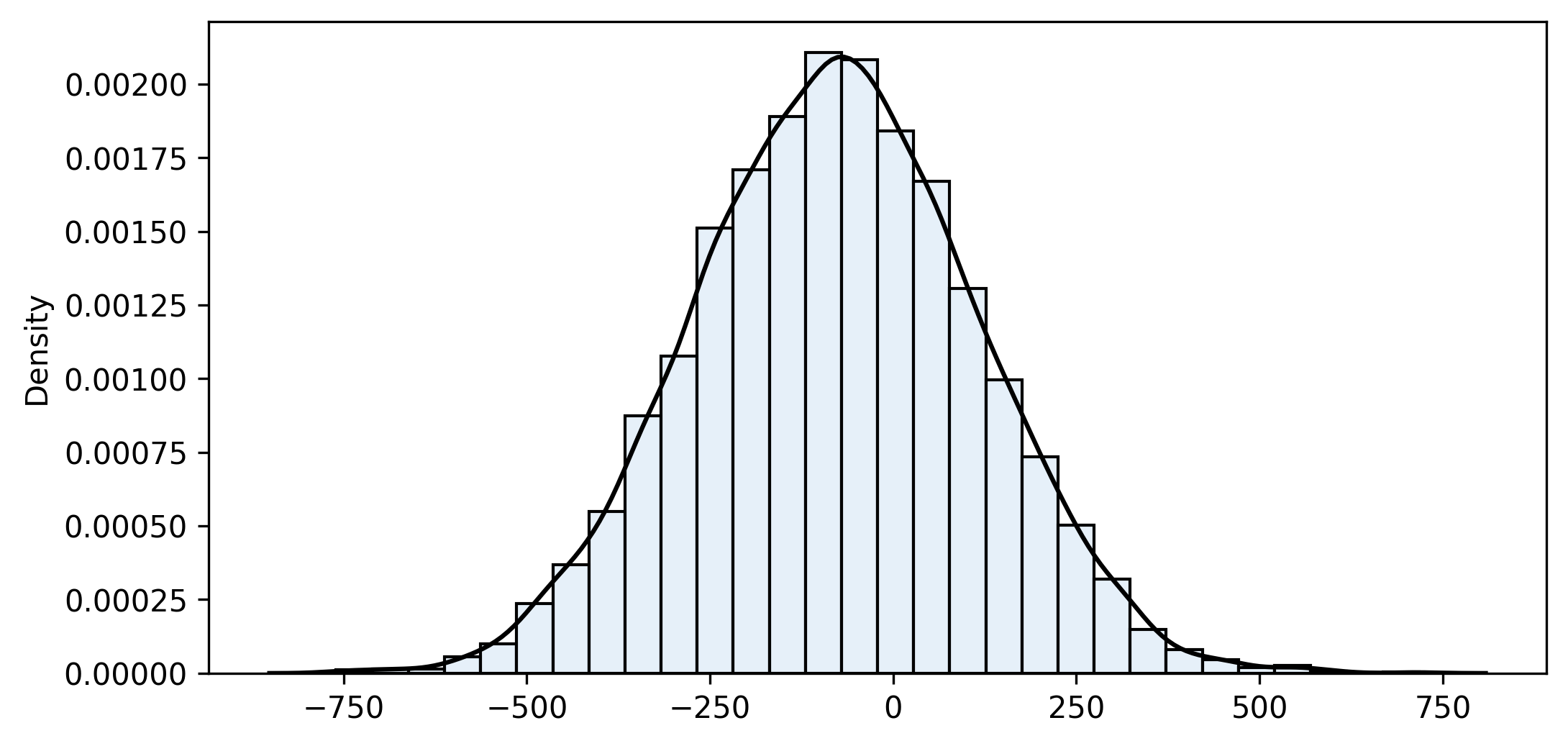

n1=75 n2=150 iterations=10000
sample_fn=-77.982 bootstrap_mean=-78.844 bias=0.862 bootstrap_se=191.647
Confidence interval (95%): [-454.325 ... -78.545 ... 296.170]

Note that the confidence interval spans from -454.325 to +296.170, so it contains 0. Consequently, we cannot disregard the possibility that there is no difference between the means. This fact leads to an interesting topic: how to use bootstrapping in hypothesis testing, which we will cover in the last article of this series.

Now we would like to go one step further. As seasoned data scientists, we are reasonably confident of landing a position in the top 30% of the corporate ladder. Consequently, we would like to narrow down our analysis to the salaries in the top quartile. At this point, there is no “traditional” parametric approach to resort to, so we apply bootstrapping. As mentioned above, we can conveniently reuse all the code except for the function that calculates the statistic. In this case, we write a new one to get the difference in means of the salaries above the 70th percentile:

from numpy import percentile

def custom_fn(x1, x2):
    """ difference in the mean of the values above percentile 70% """
    
    q1 = percentile(x1, 70)
    q2 = percentile(x2, 70)
    target1 = x1[x1 > q1]
    target2 = x2[x2 > q2]
    result = mean(target1) - mean(target2)
    
    return result
  
# bootstrap a custom statistic
bootstrap2_fn(sample1, sample2, custom_fn, iterations=10000, alpha=0.05)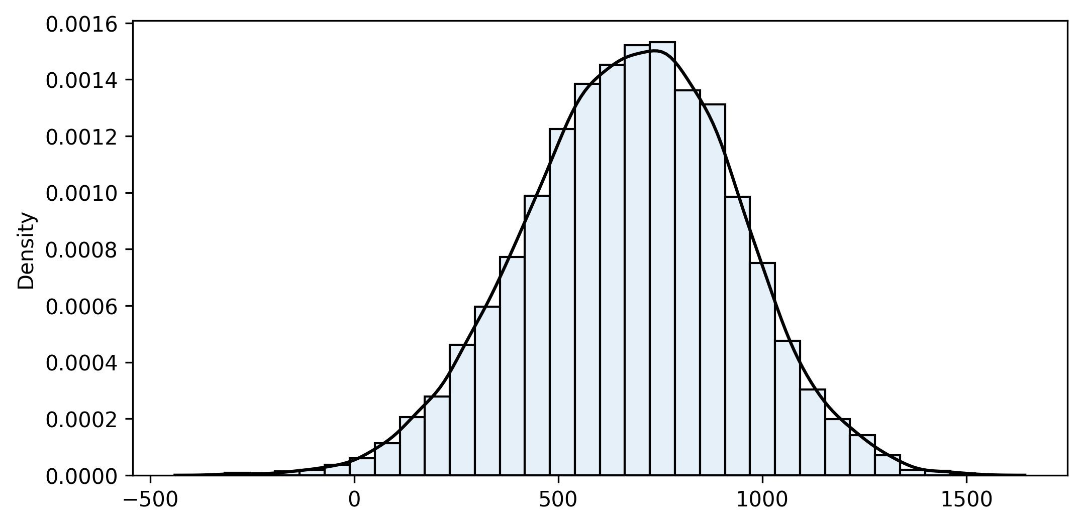

n1=75 n2=150 iterations=10000
sample_fn=680.252 bootstrap_mean=676.566 bias=3.686 bootstrap_se=256.013
Confidence interval (95%): [161.172 ... 683.415 ... 1164.408]

So we are reasonably sure (95% confidence) that company A pays more than B to the top 30% of their employees. With the given samples, that difference is estimated at 683 per month.

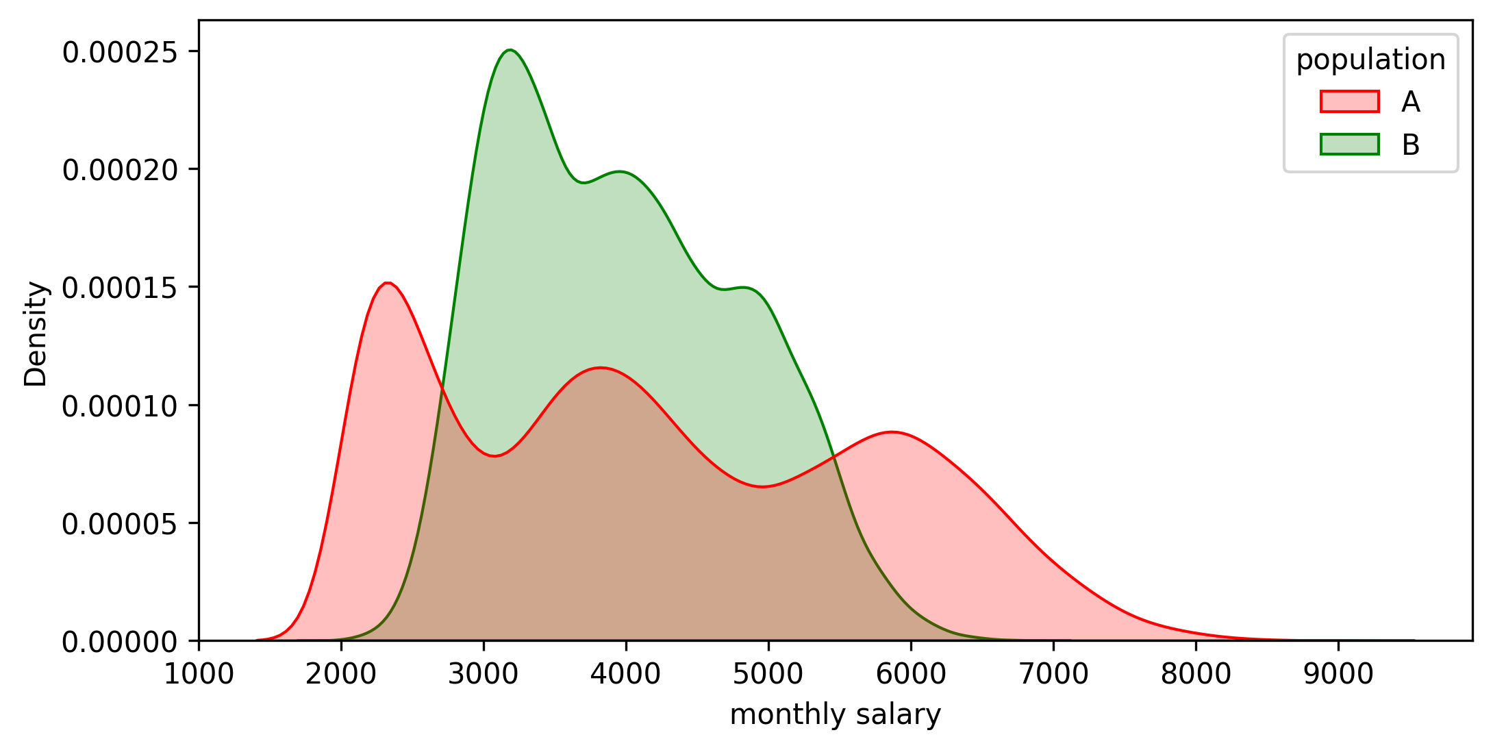
Just to double-check, let me include below the actual distributions I used to generate the samples. Both are deliberately far from normal, and their means are equal (the difference is exactly 0). However, there is a significant difference in the salaries above the 30th percentile (about 1,000). So the confidence intervals were good enough!

Final words

Bootstrapping is an elegant approach that allows us to easily build custom metrics and compare populations without prior knowledge of any theoretical framework (should it exist). We estimate a feature (or comparison of features in this case) and assess how reliable it is in the form of a confidence interval. When problems grow in complexity, parametric equations usually get more elaborate and require more assumptions to work. However, the bootstrapping algorithm remains the same, requiring minor adjustments to tailor it to the particular problem. There lies the elegance and convenience of the method.

Thank you for reading, and stay tuned for part three!

References

[1] Efron, B. (1979). Bootstrap Methods: Another Look at the Jackknife. The Annals of Statistics, 1–26.

[2] Efron, B., Tibshirani, R., & Tibshirani, R. J. (1994). An introduction to the bootstrap. Chapman & Hall/CRC.

[3] Davison, A., & Hinkley, D. (1997). Bootstrap Methods and their Application (Cambridge Series in Statistical and Probabilistic Mathematics). Cambridge: Cambridge University Press.

[4] Montgomery, D. C., & Runger, G. C. (2013). Applied statistics and probability for engineers. John Wiley & Sons.

[5] Moore, D. S., McCabe, G. P., & Craig, B. A. (2014). Introduction to the practice of statistics. Eighth edition. New York: W.H. Freeman and Company, a Macmillan Higher Education Company.