Introduction to Bootstrapping in Data Science — part 1

You know the drill: there is a population and you would like to estimate a characteristic, for example, the mean. Unfortunately, you cannot measure every individual in the population, so you draw a sample. Following the guidelines in your favourite statistics book, you simplify the problem by assuming that the parameter distribution is normal and the sample size is large enough for the Central Limit Theorem to kick in. Under these assumptions, you notice that the task at hand resembles the “Confidence interval on the mean of a normal distribution with variance unknown”, so you look up the corresponding mathematical equations, fill in the values and… job done!

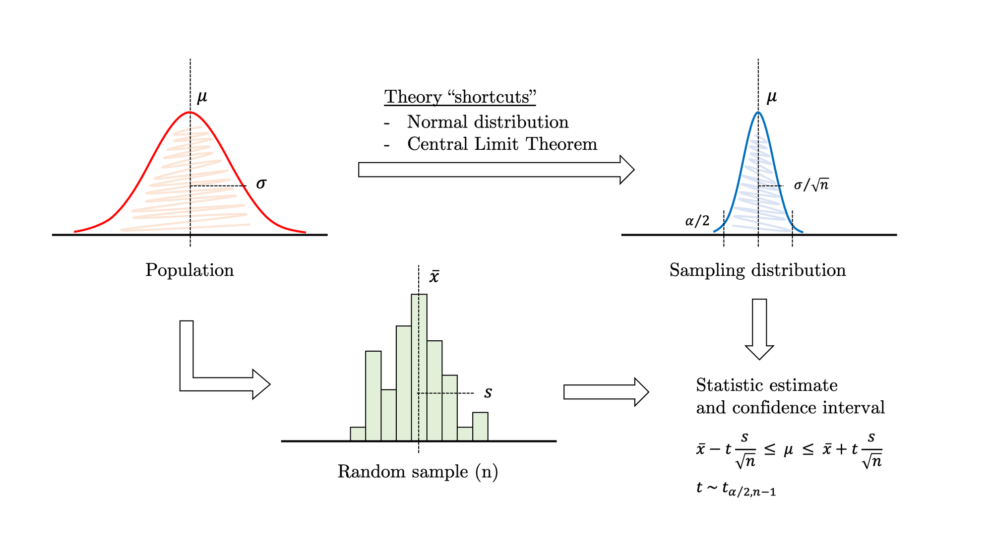
Traditional statistical methods rely on large samples, a handful of well-known theoretical distributions and the safety net of the Central Limit Theorem to work. These shortcuts allow researchers to square the circle most of the time, although this is simply impossible in certain scenarios. As data scientists, we often face challenging problems that fall outside the safe haven of traditional statistics, which is constricted to a limited number of familiar scenarios. Sadly,the reality isstubborn, data comes in all flavours of skewed shapes, and sometimes you just need to estimate parameters more complex than a simple mean.

But there is still hope. Thanks to the unstoppable evolution of computing, the study of large and complex datasets is now feasible. So are simulations that a few years ago were prohibitive to undertake. Currently, there are ways to relax some of the requisites of traditional inference and make things easier for data scientists. You can still thrive in challenging scenarios where there is not any approach sanctioned by theory.

This article gently introduces the bootstrapping method, which can be applied to almost any statistic over a sample of univariate data. The first section solves a well-known problem to set a common ground for demonstrating that bootstrapping and theoretical approaches concur. Then we move into a more complex scenario where theory is of little help and, subsequently, we address the problem with bootstrapping.

Bootstrap limitations

Before we move on, let’s tackle some misconceptions:bootstrap does not create data. What it actually does is estimating statistics, confidence intervals and performing hypothesis testing on a wide range of scenarios, even if they are not covered by the extant statistical theory. There are still some completely unavoidable limitations:

• The input must be a random sample of the population.There is no workaround around this. If the sample is not random then it is not representative, and thus the method will fail.
• Very small samples are still a problem.We cannot stretch things and create data out of nothing. Bootstrapping introduces a certain amount of variation that is intrinsic to the method. Most of it comes from the selection of the original sample and only a little from the resampling process. Consequently, the larger the sample, the better. Small samples will seriously harm the reliability of the bootstrapped results.
• Some statistics are inherently more difficult than others.For example, bootstrapping the median or other quantiles is problematic unless the sample size is quite large.

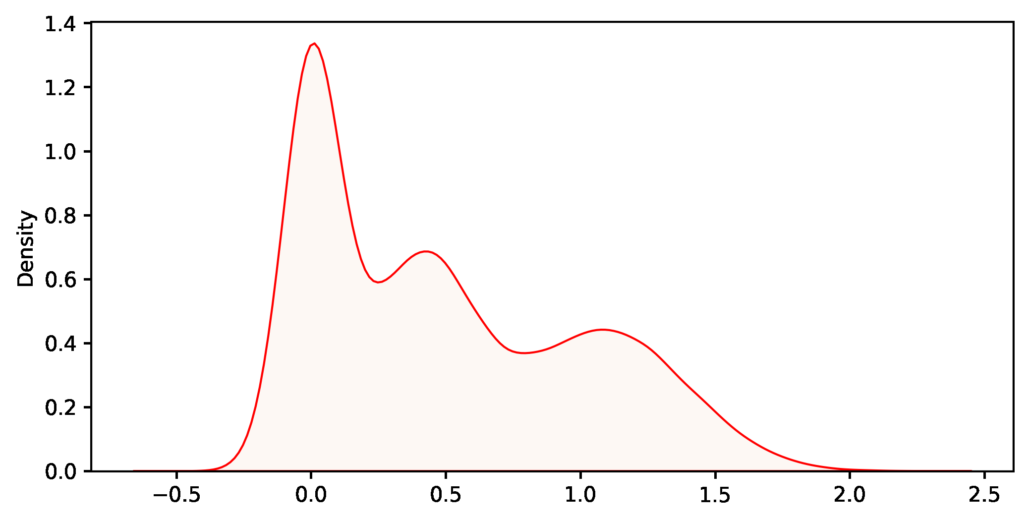
Example 1.1: traditional mean estimation

In this example, we are solving a common problem by applying both traditional and bootstrapping methods. For the population shown in figure 2, let’s estimate the mean through a random sample. As described in figure 1, this is a typical inference problem where we can safely apply the theory. Under certain assumptions, we may use the familiar expression at the right-bottom corner to calculate a confidence interval. So the process is as follows:

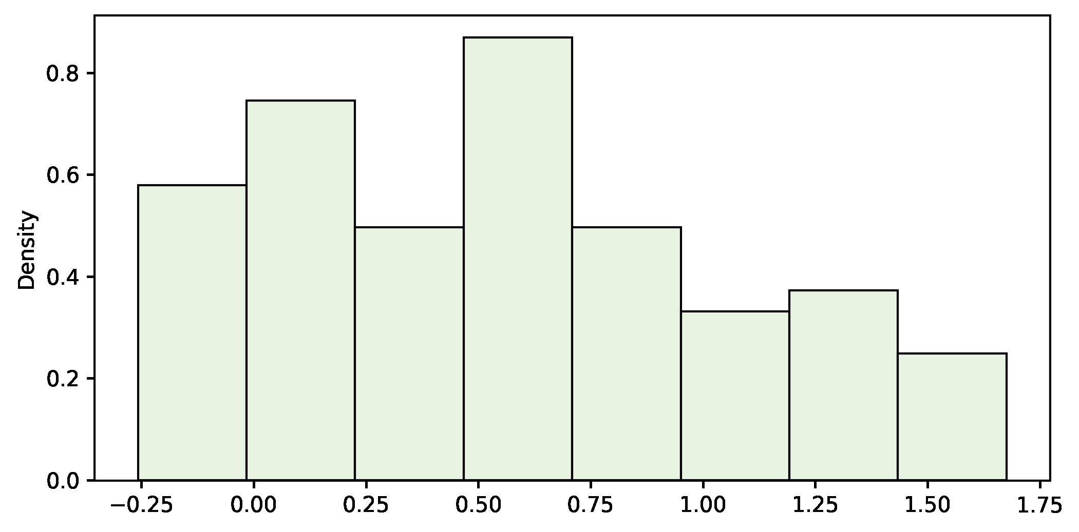
1. Take a random sample of the population (see figure 3).
2. Apply the formula with the t-statistic to calculate the interval.

# for jupyter notebooks
%matplotlib inline
%config InlineBackend.figure_format = 'svg' # ‘png’, ‘retina’, ‘jpeg’, ‘svg’, ‘pdf’

# imports
import seaborn as sns
import matplotlib.pyplot as plt
import numpy as np
import scipy.stats as st

# draw random sample
SAMPLE_SIZE = 100
sample = np.random.choice(population, SAMPLE_SIZE, replace=True)
sample_mean = np.mean(sample)
sample_std  = np.std(sample)
print(f'{sample_mean=:.3f} {sample_std=:.3f}')

# plot random sample
fig = plt.figure(figsize=(8,4))
sns.histplot(sample, color='#E2F0D9', stat='density');

# calculate mean confidence interval (step by step)
def mean_confidence_interval(data, alpha=0.05):
    n = len(data)
    m = np.mean(data)
    se = st.sem(data)
    d = se * st.t.ppf(1.-alpha/2, n-1)
    return m-d, m+d

ALPHA = 0.05
mean_confidence_interval(sample, ALPHA)

# calculate mean confidence interval (one-liner)
st.t.interval(1.-ALPHA, len(sample)-1, loc=np.mean(sample), scale=st.sem(sample))

sample_mean=0.566 sample_std=0.502
(0.46606681302580744, 0.6661796676261962)

The sample mean is 0.566, the standard deviation 0.502 and the 95% confidence interval for the population mean is [0.466, 0.666], which contains the actual value (0.500).

Example 1.2: bootstrapping the mean

One of the advantages of bootstrapping is its surprising simplicity (see figure 4):

1. Take a random sample of the population (the same as before).
2. Draw a resample with replacement from the original sample, with exactly the same size.
3. Calculate the statistic (mean, in this case) for the resample and store the result in a list.
4. Go to 2, repeat hundreds or even thousands of times.

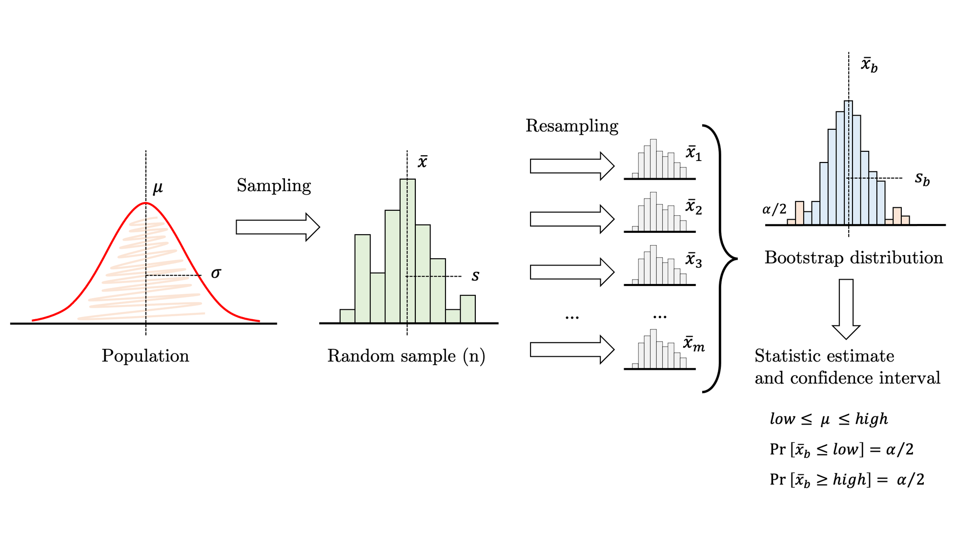
The distribution of these values is the bootstrap distribution, which should mimic the theoretical sampling distribution. Generally, it is centred on the value of the statistic in the sample (not the population), allowing for a small bias. It is always a good idea to plot it and check whether it is approximately normal. If it is, you may revert to a traditional t-statistic and this approach is known as bootstrap-t. Otherwise, just compute the non-parametric bootstrap percentile confidence interval, that is, pick the two quantiles that enclose under the bootstrap distribution the area required for your confidence level. The second approach is impervious to skewness, so it is usually more accurate as long as the bias is small.

Bootstrapping is a technique that works pretty well. However, if you get a relatively large bias or the bootstrap distribution deviates noticeably from normal, those are two clear symptoms that the procedure may not be working as expected. In that case, you should proceed with caution.

def bootstrap_fn(sample, fn, m, alpha):
    """ bootstrap a given function """
    
    n= len(sample)
    sample_fn = fn(sample)
    
    # bootstrap algorithm
    bootstrap_dist = []
    for i in range(m):
        resample = np.random.choice(sample, n, replace=True)
        estimator = fn(resample)
        bootstrap_dist.append(estimator)
    
    # calculate mean, standard error and bias
    bootstrap_mean  = np.mean(bootstrap_dist)
    bootstrap_se    = np.std(bootstrap_dist)
    bias = sample_fn - bootstrap_mean
    
    # calculate bootstrap percentile confidence interval
    percentile_high = 100 * (1-alpha/2)
    percentile_low = 100 * (alpha/2)
    high   = np.percentile(bootstrap_dist, percentile_high)
    median = np.percentile(bootstrap_dist, 50)
    low    = np.percentile(bootstrap_dist, percentile_low)
    
    # print results
    print(f'Bootstrap results:\n {n=} {m=} {sample_fn=:.3f} {bootstrap_mean=:.3f} {bias=:.3f} {bootstrap_se=:.3f}')
    print(f'Confidence interval {1-alpha:.0%}:\n [{low:.3f} .. {median:.3f} .. {high:.3f}]')
    
    # plot bootstrap distribution
    fig = plt.figure(figsize=(8,4))
    sns.histplot(bootstrap_dist, color='#DEEBF7', stat='density')
    sns.kdeplot(bootstrap_dist, color='black')
    
# bootstrap the mean
ITERATIONS = 1000
bootstrap_fn(sample, fn=np.mean, m=ITERATIONS, alpha=ALPHA)

Bootstrap results:
 n=100 m=1000 sample_fn=0.566 bootstrap_mean=0.567 bias=-0.001 bootstrap_se=0.049
Confidence interval 95%:
 [0.471 .. 0.566 .. 0.670]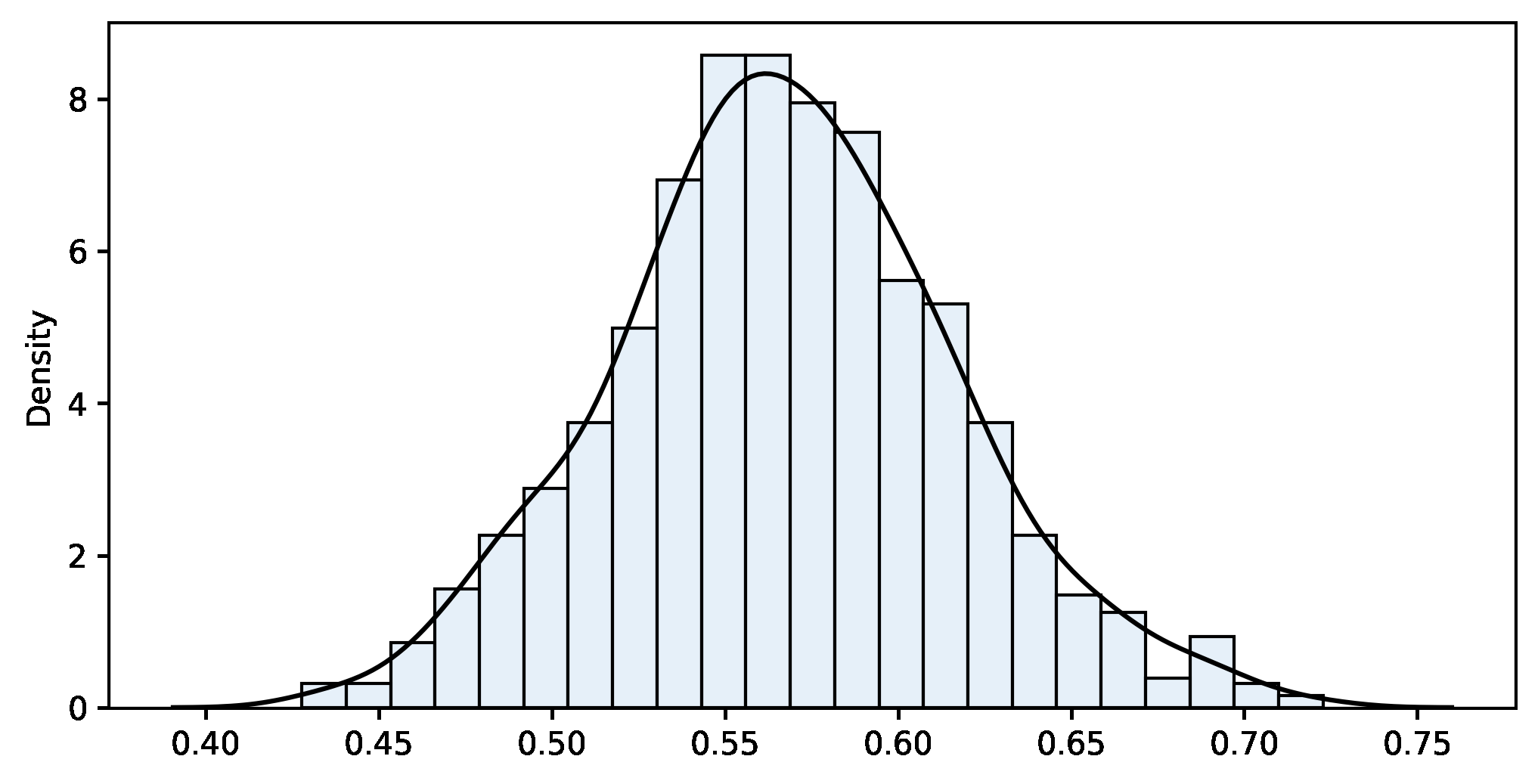

If we compare with the traditional approach, both results are pretty close. Again, let’s stress that bootstrapping does not create data. It is a way to move forward without the theoretical support of a sampling distribution. We use the bootstrapping results for two purposes: estimating a parameter and its variability. We don’t need to make theoretical assumptions such as the normality of the population nor rely on the Central Limit Theorem. This approach works even if the theory does not explain the sampling distribution of our statistic (more on this in the next example). The bootstrap distribution (see figure 5) fills that gap and allows us to estimate confidence intervals directly from it.

Example 2: the average of the top 50%

We would like to calculate the average of the individuals in the top 50% of a population. In other words, the mean of the values above the median. This custom parameter is not as common as the mean, and consequently, you will not find any hint in your textbook to estimate it. Without a theoretical approach, we have to resort to bootstrapping.

Thanks to the Plug-in principle, we may estimate almost any attribute of a population by calculating the same attribute on a sample drawn from it. Bootstrapping will take care of the rest, providing us with the appropriate bootstrap distribution to approximate everything else.

The procedure is exactly the same as before with just a slight change: we have to replace the mean with the new statistic. Therefore, we write a new function and reuse the rest of the code.

def custom_fn(x):
    """ mean of the values above the median """
    median = np.median(x)
    top = x[x > median]
    result = np.mean(top)
    return result

# bootstrap again, replace mean by custom_fn
bootstrap_fn(sample, fn=custom_fn, m=ITERATIONS, alpha=ALPHA)

Bootstrap results:
 n=100 m=1000 sample_fn=0.979 bootstrap_mean=0.981 bias=-0.002 bootstrap_se=0.067
Confidence interval 95%:
 [0.850 .. 0.983 .. 1.112]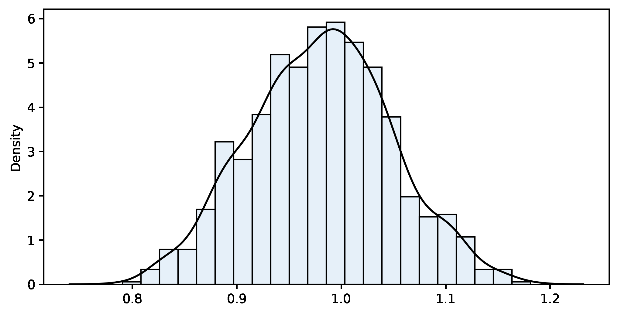

The result is quite good because the actual value of the mean of the top 50% is 0.902, well within the provided interval. In a blink of an eye, the computer has run a thousand iterations to build the bootstrap distribution and calculated the confidence interval of a novel statistic that was not available in our textbooks. This is a good example of the power and convenience of the method.

Final words

The alleged origin of the word bootstrapping is a passage from one of the editions of “The Singular Adventures of Baron Munchausen” (1786) when the main character gets out of a hole by pulling the straps of his own boots.

This metaphor applies to some extent: while bootstrapping does not create data, this simple computational technique allows us to go one step farther with the data at hand, and it works even when theory is not available or assumptions cannot be safely made.

There is a wide range of bootstrapping applications that I cover in subsequent articles (see below). If you are interested in the topic, I strongly recommend you to have a look at the references. Thank you for reading!

References

[1] Efron, B. (1979). Bootstrap Methods: Another Look at the Jackknife. The Annals of Statistics, 1–26.

[2] Efron, B., Tibshirani, R., & Tibshirani, R. J. (1994). An introduction to the bootstrap. Chapman & Hall/CRC.

[3] Davison, A., & Hinkley, D. (1997). Bootstrap Methods and their Application (Cambridge Series in Statistical and Probabilistic Mathematics). Cambridge: Cambridge University Press.

[4] Montgomery, D. C., & Runger, G. C. (2013). Applied statistics and probability for engineers. John Wiley & Sons.

[5] Moore, D. S., McCabe, G. P., & Craig, B. A. (2014). Introduction to the practice of statistics. Eighth edition. New York: W.H. Freeman and Company, a Macmillan Higher Education Company.