All Mushrooms Are Edible, But Some Only Once
A visual introduction to the confusion matrix and classification metrics.

The problem
Some time ago, a Biology professor told me that “All mushrooms are edible, but some only once.” Putting aside scientists’ dark sense of humor, mushrooms are a great example to illustrate the intricacies of classification problems and to introduce the performance metrics typically applied in this context.
The situation is the following: as it is widely known, some mushroom varieties are a delicacy, while others are toxic and may even cause death. As expert data scientists, wouldn’t it be great to train a machine learning model to identify poisonous mushrooms automatically? In the end, it is just a binary classification problem: poisonous (the positive case) or edible (negative).

Before anything else, we need a labeled dataset consisting of a large enough number of mushrooms for which we already know the proper classification. Hiring an expert mycologist would definitely come in handy during this project phase.
The next step is to split the dataset into the training and test sets.A reasonable division would be 70% training and 30%test.However, other divisions are also fine depending on the number of observations available and the proportion of each class.
Training a model is not easy. In this case, the input variables are the features of each mushroom, and the output or target variable is the desired classification into poisonous or edible.At this point, it is essential to stress that the model must be trained solely on the training set and evaluated on the test set. Since designing and fitting models are not in the scope of this article, let’s skip this part and assume that… Voilà! The model is ready.

Now we come into the exciting part. How good is the model? To answer this question, we use it to predict whether the mushrooms in the test set are poisonous or not. While we already know the answer, the model has not seen those before. Consequently, by comparing the predicted and actual values, we can measure the classification performance and the ability to generalize.
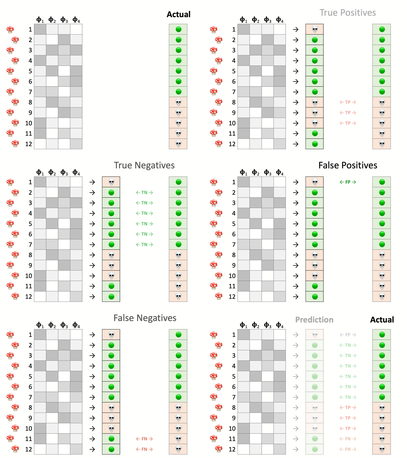
Testing the model and measuring performance
Here we have a test set that consists of 12 mushrooms. Their corresponding features are on the left side, and the rightmost column indicates whether they are poisonous or edible. Next, we make predictions with our model. Comparing the predictions in the center and the actual values on the right, we find that the model correctly classifies some instances while committing errors in others.
When the model accurately classifies a poisonous mushroom (the positive case), it is called a True Positive. Similarly, the correct identification of an edible mushroom (negative) is a True Negative.
Those are the correct answers, and then there are some mistakes. A False Positive occurs when the model labels an edible mushroom as poisonous. Conversely, a False Negative is a poisonous one mistakenly classified as edible. These are also known as Type I and Type II errors, respectively.
Not every mistake is the same, though. The severity depends on the specific details of the problem at hand. For example, a false negative is much worse than a false positive in our case. Why?

A false negative means that a poisonous mushroom was incorrectly identified as edible. That is a severe health hazard as it could potentially have harmful or even deadly consequences. Conversely, a false positive, or classifying an edible mushroom as poisonous, has no real repercussions apart from discarding food in perfect condition and throwing it in the trash.
The Confusion Matrix
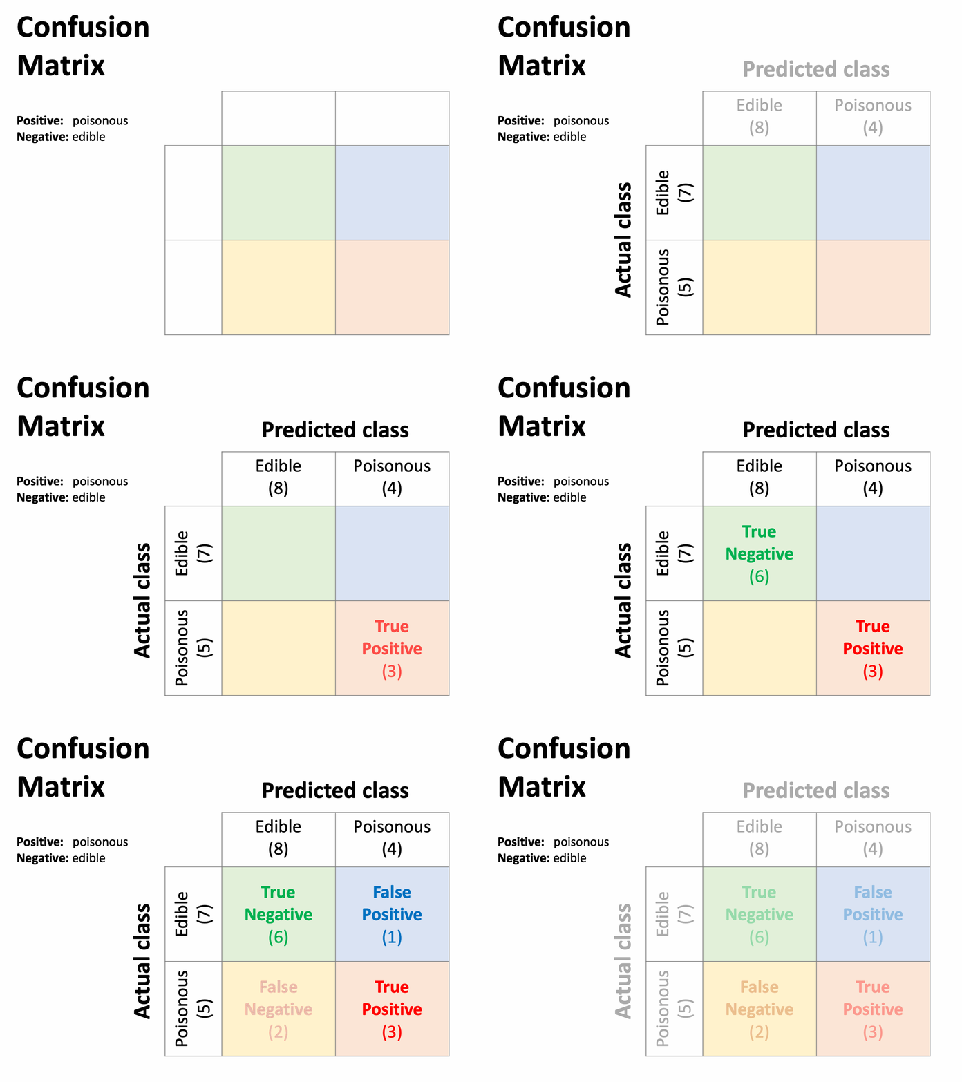
These results can be displayed in a table with a specific layout known as the confusion matrix. The horizontal rows represent the observed classes, while the columns show the predicted classes. In a binary classification problem, they intersect in four cells that outline every possible outcome.
The correct classifications are shown in the diagonal, while the errors are displayed outside. This allows finding where the model confuses two classes (hence the name). Be aware that this matrix may appear transposed in many documents and software packages, that is, the predictions in rows and actual values in columns. Both variants are common in the literature.
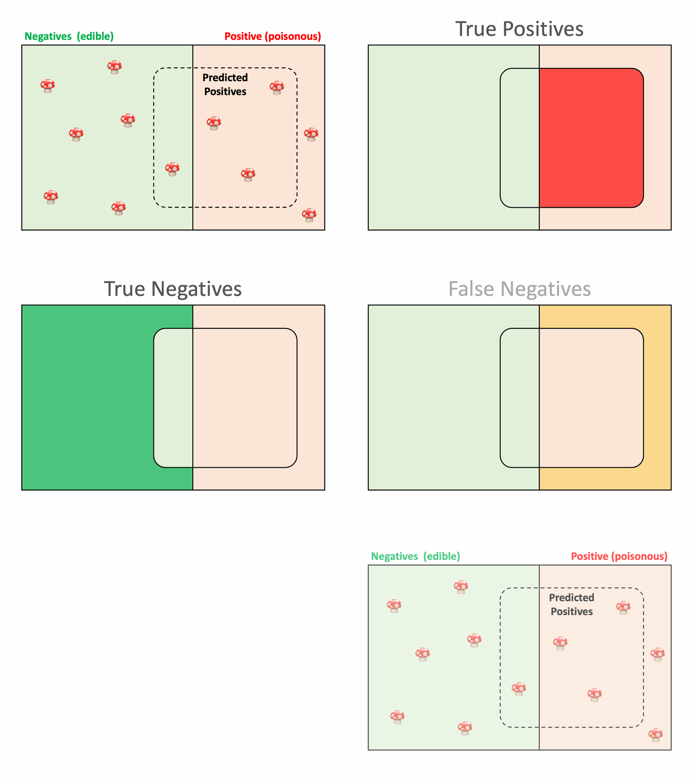
Another way: a Venn diagram
We can illustrate these outcomes with a Venn diagram. The actual classes appear in the rectangular area in the background. Next, we surround the predicted positives with a dotted curve. The individuals inside this region are the ones that the model identified as poisonous. The best case would be for this region to overlap with the red area perfectly, as that would mean that the model classifies every mushroom correctly. Unfortunately, this is not happening in the example.
While the confusion matrix and the Venn diagram are great tools to visualize how well the model performs, it would be awesome to synthesize the performance into a single numerical value. As classification is a multifaceted problem, many metrics are available, each one focusing on a specific aspect. Let’s have a closer look at some of them.

Sensitivity, Recall or True Positive Rate (TPR)
How well can the model detect poisonous mushrooms?
In other words, sensitivity is the ratio of true positives divided by the observed positives.
Sensitivity is the metric of choice when the top priority while training the model is capturing as many positives as possible (our example).

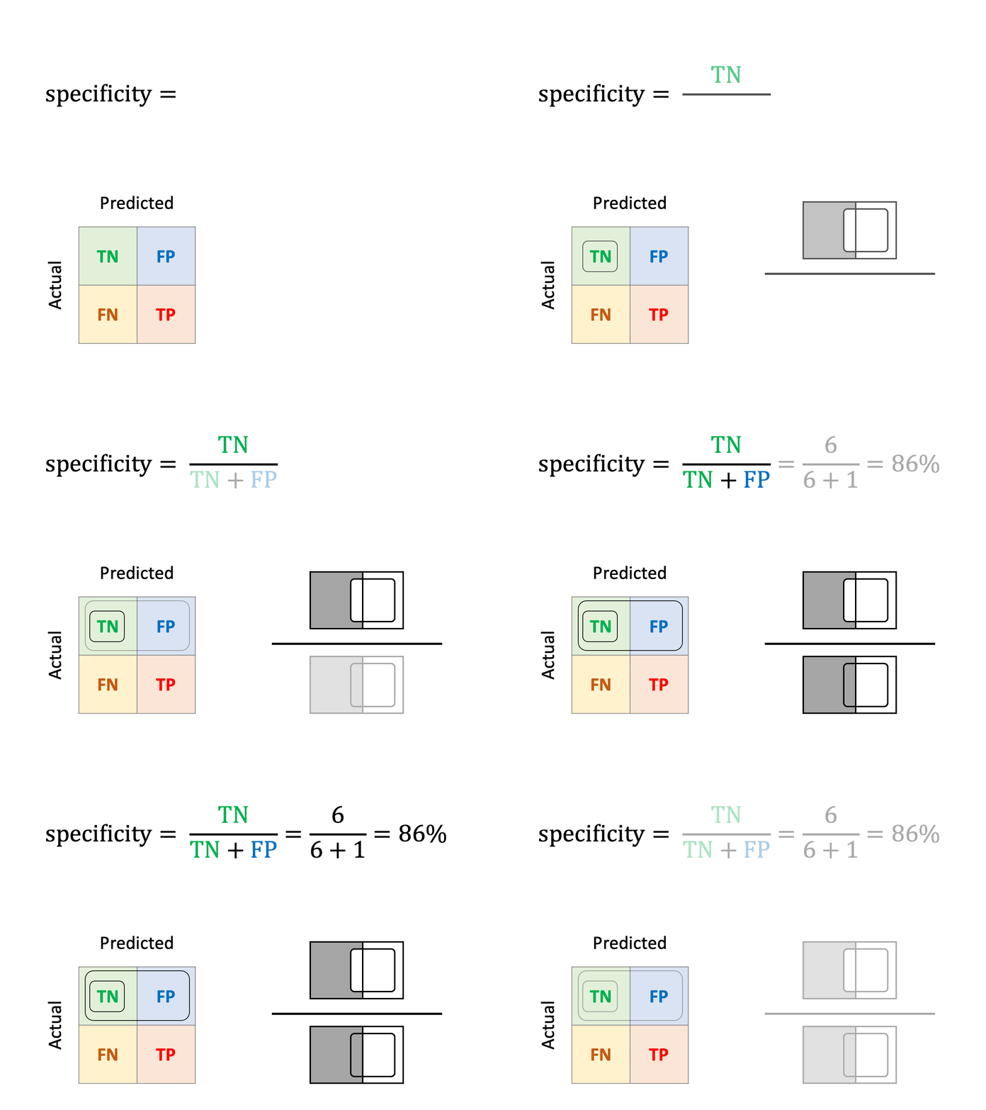
Specificity or True Negative Rate (TNR)
How well can the model detect edible mushrooms?
Likewise, specificity is the ratio of true negatives divided by the actual negatives.
Specificity is a proper choice when the occurrence of false positives is undesirable, as if we wish to monitor closely how many edible mushrooms are thrown away.
Precision or Positive Predictive Value (PPV)
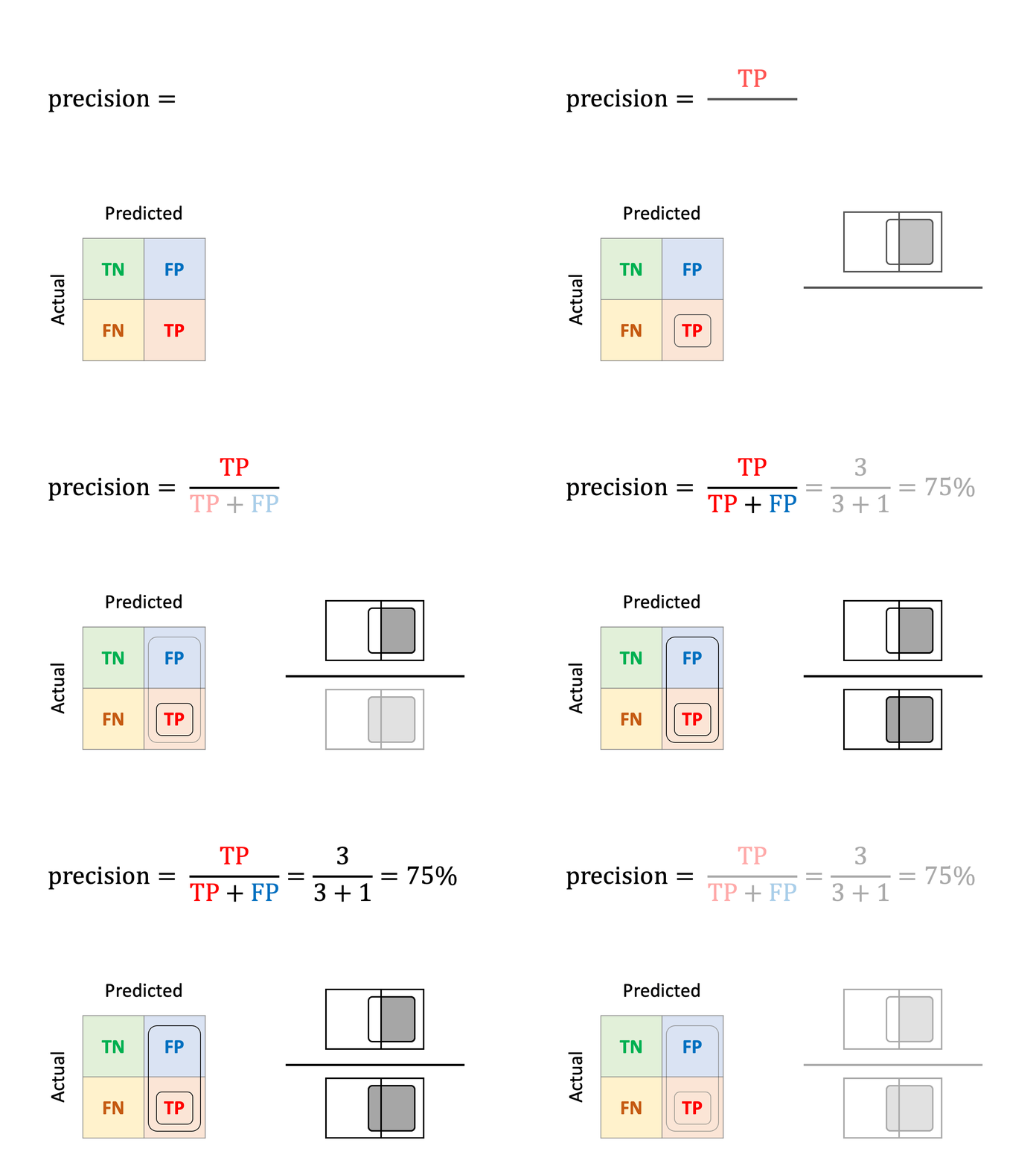
What fraction of mushrooms predicted as poisonous are really poisonous?
While sensitivity and specificity focus on observed classes, some metrics measure the performance of predictions. For instance, precision is the ratio of true positives over predicted positives.
Precision is the metric that should be monitored if you wish to be confident in the predicted positives.
Accuracy
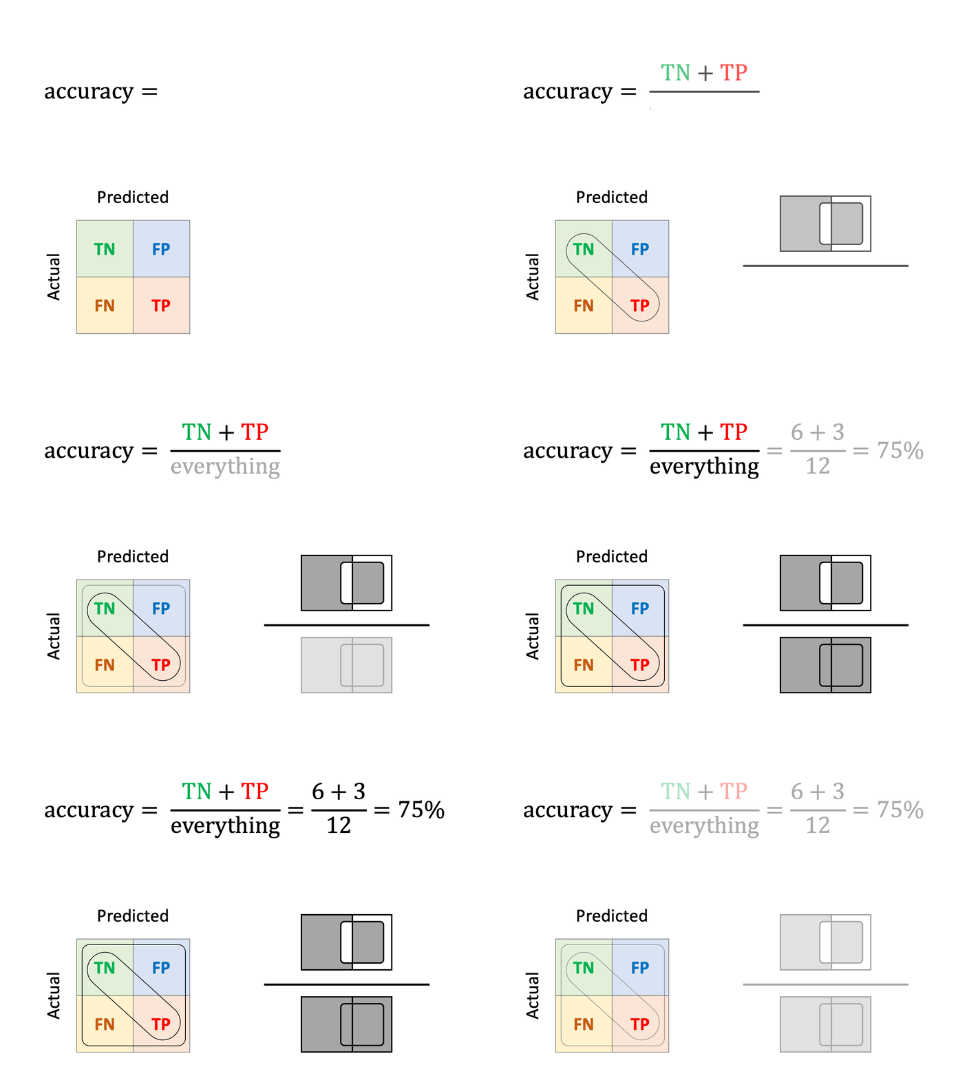
What is the fraction of correct classifications?
A unique metric that simultaneously measures both true positives and negatives should be useful. Unfortunately, accuracy provides misleading results in problems with unbalanced classes.
If you need to synthesize a classifier’s overall performance in a single value, have a look at metrics such as balanced accuracy, F1 score, or the Area Under the Curve (AUC).
Naïve model: the majority rule
We have gone to great lengths to build a model, but how can we ensure it is worth the effort? Are the predictions of any value? Is using the model any better than having no model at all?
To answer this question, we must confirm that the model provides enough information to justify its existence. Model selection is a task complex enough to deserve a dedicated post; however, let’s have a glimpse at the topic and briefly introduce the concept of a naïve model: an unsophisticated model that delivers a prediction without leveraging any of the input data at its disposal.
A sound choice for a naïve classification model is the majority rule. It ignores the input variables and labels every individual as the most frequently observed class in the training set (negative or edible in our example). This model is inexpensive to build and should be correct more times than not. Specifically, the accuracy of this model, also known as no-information rate, is the proportion of the majority class in the training set.
Every model must beat this benchmark to be significant. Otherwise, operating it is pointless, and we should either stick to the superior naïve model or go back to the design table and rethink our approach.


Conclusion
Binary classification is a common technique that every data scientist should master as it lies at the core of many business and scientific problems. A good grasp of this foundation is also crucial as multiclass classification extends and generalizes these concepts. The more tools you have in your data science toolbox, the better equipped you will be to face new and challenging problems.
I hope you found this article useful… and be careful with mushrooms!


